
“Simple Linear Regression in Python for Machine Learning”
“Simple Linear Regression in Python for Machine Learning”

How would you define simple linear regression?
Simple linear regression is a statistical method used to model the relationship between two variables by fitting a straight line to the data. One variable is considered independent (predictor), and the other is dependent (outcome). The goal is to predict the dependent variable based on the value of the independent variable using a linear equation. The relation between the variables may be defined as
y=mX+c , Here’s a breakdown of each term:
- y: The dependent variable, which is the value we are trying to predict.
- X: The independent variable, which is the value used to make the prediction.
- m: The slope of the line, representing the rate at which y changes with respect to X. It shows how much the dependent variable is expected to change for a one-unit increase in the independent variable.
- c: The y-intercept, which is the value of y when X is zero. It indicates where the line crosses the y-axis.
Together, this equation describes a straight line that best fits the data, allowing us to make predictions about y based on different values of X.
How to perform a simple linear regression?
To demonstrate how to perform simple linear regression using Python, we’ll use the scikit-learn library, which provides easy-to-use tools for regression models.
Steps:
- Install necessary libraries.
# Step 1: Import necessary libraries

import seaborn as sns
import numpy as np
import pandas as pd
import matplotlib.pyplot as plt
from sklearn.model_selection import train_test_split
from sklearn.linear_model import LinearRegression
from sklearn.metrics import mean_squared_error, r2_score
2. Import and prepare the dataset.
We will use Iris dataset in this example.
# Step 2: Prepare the dataset

iris=sns.load_dataset('iris')
iris=iris[['petal_length','petal_width']]
X=iris['petal_length']
y=iris['petal_width']
We need to have some correlation between variables to perform linear regression. Lets find out the relation using graph
plt.scatter(X,y)
plt.xlabel('Petal Length')
plt.ylabel('Petal Width')
plt.show()
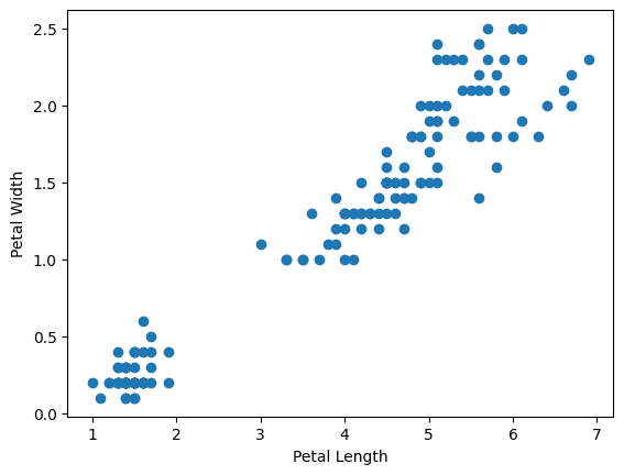
Here we have some good positive correlation between X and y
3. Split the data into training and testing sets.
For machine learning we have to split the dataset into training and test sets
#Step 3: Split the data into training and testing sets

X_train,X_test,y_train,y_test=train_test_split(X,y,test_size=0.4,random_state=42)
For sklearn linear regression the data should be two demensional so we reshape our data
X_train=np.array(X_train).reshape(-1,1)
X_test=np.array(X_test).reshape(-1,1)
4. Fit a simple linear regression model.
# Step 4: Fit the simple linear regression model

lr=LinearRegression()
results=lr.fit(X_train,y_train)
5. Make Predictions.
# Step 5: Make predictions
y_pred=lr.predict(X_test)
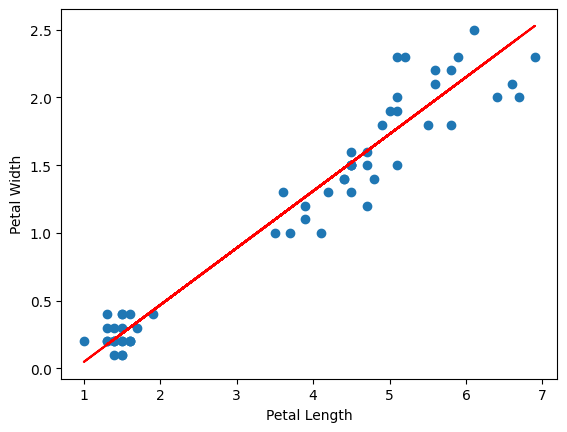
6. Visualize the results.
# Step 6: Visualize the results

plt.scatter(X_test,y_test)
plt.plot(X_test,y_pred,color='red',label='Regression Line')
plt.xlabel('Petal Length')
plt.ylabel('Petal Width')
plt.show()
7. Evaluate the model.
We will use MSE(Mean Squared Error) and R-squared score matrices to evaluate the model
# Step 7: Evaluate the model
mse = mean_squared_error(y_test, y_pred)  # Mean Squared Error
r2 = r2_score(y_test, y_pred)  # R-squared score (goodness of fit)
# Print the slope and intercept
print(f"Slope (m): {lr.coef_[0]}")
print(f"Intercept (c): {lr.intercept_}")
print(f"Mean Squared Error: {mse}")
print(f"R-squared: {r2}")
#Output
Slope (m): 0.42061482666301725
Intercept (c): -0.3736970002822666
Mean Squared Error: 0.03720338284196041
R-squared: 0.9381204129407422
Conclusion:
The simple linear regression model has successfully established a relationship between the independent and dependent variables. With a slope (m) of 0.4206, the model suggests that for every unit increase in the independent variable, the dependent variable increases by approximately 0.42 units. The intercept © of -0.3737 indicates that when the independent variable is 0, the predicted value of the dependent variable would be -0.37.
The Mean Squared Error (MSE) of 0.0372 indicates that the model’s predictions are, on average, only slightly off by a small margin, which demonstrates good predictive performance. Moreover, the R-squared value of 0.9381 shows that about 93.81% of the variance in the dependent variable is explained by the independent variable, indicating a strong fit of the model.
In conclusion, the model performs well with high accuracy, but there is still a small portion of variability in the data that is not explained by the model, which may require further investigation or the inclusion of additional factors.